The following is an old paper I wrote about 20 years ago on electronically modeled neurons and how they may be used to approximate functions in various topologies. The paper won’t go into highly complex cases of pattern recognition; yet it describes a possible basis to a greater multi-dimensional function approximation model.

This paper wasn’t the winning paper for a noble prize 😉 but it may be of value to someone considering “unorthodox” neural networks, even if just for the fun of it. Today we have much more powerful computers than we had access to back then. I am certain much more could be achieved with this type of method today given that computational power has grown far beyond what we had in the mid-1990s.

Introduction

             As continuation of previous papers, the current research status involves one-dimensional function approximation using frequency domain neurons. Frequency Domain Neurons (FDN) are utilizing complex arithmetic, which is very economical on today’s digital computers.

            The system’s input information is encoded as a sinusoid frequency, or complex vector, with constant amplitude (in complex math terms: magnitude) for simplicity. The whole networks acts then as a single huge complex vector on the input that can be interpreted as a elaborate “band-pass” in electrical terms.

            Examples (sample points) of the desired goal function (the function itself is usually unknown) are given to the network, and a Genetic Algorithm (GA) adapts to the goal function. It finds the optimal number of neurons and the internal structure of the network necessary to best approximate a function going through the sample points.

            Of course, there are many other ways to approximate one-dimensional functions with quite good accuracy, why then use this particular method? The inspiration to use low-pass neurons really originated from preceding steps of the ongoing research. Biological neurons act as low-pass filters on the input and therefore perform a complex multiplication on the input signals. The outputs of the GA presented here in this course could be used as an example of how brain cells could approximate “complicated” functions in real life. The second reason for using this particular method is that training and using a FDN is by far much more efficient when considering digital computation platforms. Additionally, conventional Artificial Neural Networks (ANN) involve more intensive computation and much more examples for training than FDNs.

Why Not Use Artificial Neural Networks?

            Conventional ANNs use, usually natural exponent-based activation functions (also: transfer functions). Two examples for the most popular ones are as follows:

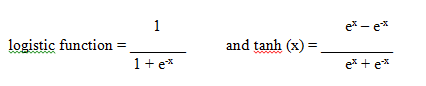
            As you can clearly see, enormous computation has to be performed to compute just the activation function of each neuron. During training, conventional ANNs algorithms even require N³ computations of this functions because of their multi-passing inside the network O(N³). Also, neurons are structured in layers, each layer fully interconnected with the previous layer. Each neuron is fully interconnected with all neurons of the previous layer with weights (floating point numbers). Evaluating the network’s output involves then N² computations of weighted-sum and activation function outputs.

            Another reason for not using numerical ANN methods is that they numerical simulations and thus not deterministic. As we will see later, FDNs approximate functions as a single multivariable complex vector that can be easily found through symbolic calculations. Thus FDNs are fully deterministic functions that allow them to be used even for mission-critical applications, since all states are known and predictable.

            The structure of ANNs is also fixed in order to make the training algorithms simpler. However, a fixed structure is obviously not going to cover many training problems optimally. Also, how does a user know how many neurons are necessary? So far, there is no proven mathematical method to answer that question.

 

Frequency Domain Neural Networks

            FDNs are cellular complex arithmetic systems having a transfer function that is multiplied on the input vector. The author has used so far normal low-pass filter vectors and a combination of low-pass filters: the band-pass filter function.

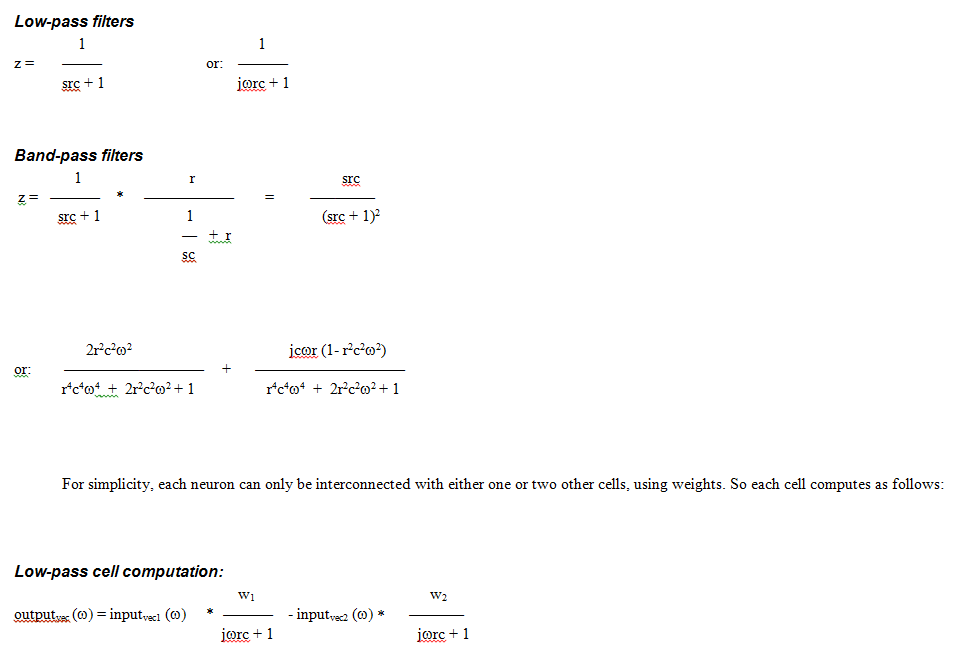
Band-pass cell computation:

        

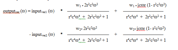
            For each network, there is one input source and an unlimited number of cells connecting to each other and/or the input source. The structure is absolutely free, as long as there are no feedback paths in the circuit.
Electrically “speaking” each neuron has the following schematic:

 

 

Figure 1.1. This is a Frequency Domain Low-Pass Neuron.

 

 

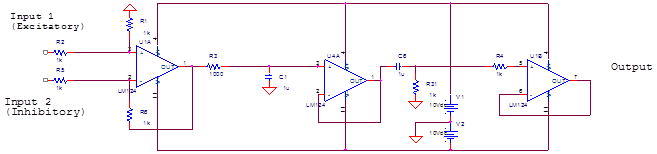
Figure 1.2. This is a Frequency Domain Band-Pass Neuron.

            When the output of the network is investigated, the magnitude of the input vector is examined and shown as spectral diagram (see GA output of following section).

How to Train a Frequency Domain Network

Since a FDN network is full of hundreds of open variables (Rs, Cs, weights, structure of interconnection, etc.), a Genetic Algorithm was written to develop optimized networks fitting the desired goal function. The GA method was as follows:

1.    Generate a random population of a random number of neuron for each individual, randomly parametrized and interconnected.

2.     Evaluate the fitness for each cell inside of each individual network and sort results ascendingly.

3.      Take N best cell branches and copy them recombined into a new generation, consisting of M new individual networks.

4.      Add more random individuals (cellular networks) to the population.

5.      Mutate these new individual networks by some probability.

6.     Go back to step 2.

The computer program was written in C++, allowing dynamic allocation of objects. Each frequency domain neuron was designed as an object, dynamically growing and changing structures were set up with pointers from object to object. A population object was designed that controls all Assembly objects and performs the GA steps on them. The reader can run the program on disk to see how the network’s output function approximates the goal stepwise.

One interesting phenomenon of the program is that the user can see visually how the GA runs into sub-optimal solutions and how the mutation of networks helps to get out of them. Also, by adjusting the parameters, the user can see the impact of the maximum number of neurons used, weight range, R and C range, probability of mutation, etc.

            Here are some sample GA transitions showing how GAs approximate a function. The goal function used here is sqr (x).

 

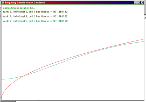
Figure 1.3. These are screen shots from the GA’s spectral output. The x-axis represents frequency and the y-axis shows the vector attenuation. Goal function (in red) was f(x) = sqr (x / 50) with 200 equally distributed sample points. The fitness was evaluated as sum of |Netoutput (x) – f(x)|², the Mean Square Error. The other two or three curves show the second, third, and fourth best curve of a particular generation. These results printed here are by far not perfect. The parameter ranges, such as weight-range, R and C range, etc. have not been optimized at all. These results were obtained rather by guessing and trial-and-error of the ranges for a few times.

             It was found that low-pass filter transfer functions are good approximators for continuous functions with always equal-signed first derivative, such as f(x) = x, sqr (x), 1 / x, etc. For sine-wave or fluctuating functions, it is more efficient to use band-pass filter transfer functions. The reason for this is quite obvious: band-passes of higher quality (cascaded band-passes) have a bump-like spectral shape that sharpens with increasing band-pass quality. Given that enough cells are available, summing band-pass filter outputs together can approximate any sequence of consecutive samples.

 

Band-Pass Filter Assemblies Can Approximate Any Function

            Consider the following graph:

 

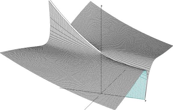
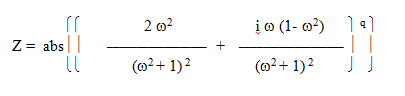
Figure 1.4. This graph shows the output vector magnitude of a band-pass (center frequency = 1Hz) when a unit-vector of increasing frequency is inputted. The Z axis represents the magnitude of the vector, frequencies (w) run on the X-axis, and the Y axis increases the band-pass quality. The band-pass quality is the exponent of  the band-pass transform vector, which has the following form:

                    

            As you follow figure 1.4 the left to the right (neg. Quality towards pos. Quality), you can clearly see that the band (follow X-axis) at 1Hz gets increasingly narrower. In the negative half of the Y-axis, the band-pass function is reversed into a notch-filter. Inside that region, the band-pass actually amplifies the band.

Learning & Function Approximation

            The “ideal” learning machine has to adapt quickly to additional examples. Examples in this and many other models are mathematically speaking points on an unknown curve. For simplicity, we only cover one-dimensional dependencies in this paper. In other words, there is only one independent variable controlling causing a certain effect, which is the learning curve. Then, learning refers to quickly finding a curve or equation that goes through all the sample points given.

The strength of the model introduced in this paper is that using complex vectors or filters as neurons allows very quick adaptation without the need to reorganize the whole “memory” or structure of the learning system. Also, the system shown here is not permanently growing: It was found in many experiments that linear combinations of complex-vector neurons offer still a compact solution to any given problem curve.

            For example, one could use as well the Discrete Fourier Transform or polynomial curve fitting methods to approximate a curve by samples. However, with every additional sample introduced to the learning system one would have to train the whole network again. The result would be that for each additional point in the curve, the structure has to be changed completely, especially when relative outlyers have to be included to the learning curve.

Imagine multiple band-passes as shown in figure 1.4 added together using different center frequencies (the center frequency can be adjusted by the changing R and C constants). The output curve could then approximate any shape along the X-axis:

   

 

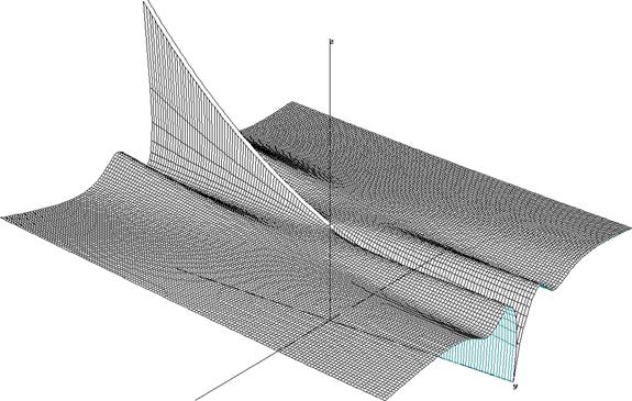
Figure 1.5. Just one band-pass was added to the function used in figure 1.4 to illustrate how linear combinations of band-passes look visually. The second band-pass has a center frequency 7.7Hz.

Conclusion

            The filter solution to adaptive learning problems presented here allows devices to adapt to large-scale inputs without the need of reorganization. The Genetic Algorithm used to evolve networks that fit to any problem universally, automatically optimize the network, given that mechanisms are provided to the GA to do so.

            The future of Neural Networks is clearly focusing on adaptation and dynamic growth, since it became obvious in the last decade that fixed-structured or predetermined network organization is unable to cope with large-scale input requirements. Also, the speed of such systems is a critical point why many industries reject ANNs.

            The future is also seen in digital systems, because they are (virtually) absolutely predictable. The method presented in this paper gives users the possibility to derive a complete equation for a given network. If dynamic growth is not necessary, one can program a low-cost digital CPU to evaluate the equation instead of numerically computing complex vectors. In that sense, the fields of application of this method are very broad and promising.

            However, there is much to do on implementation issues as well as on the mathematics of this approach. One major step to follow is clearly the adaptation of multi-variable systems or learning curves. Implementation issues include business connections, and specific knowledge of meaningful application fields.

Acknowledgements

            The author wants to use this opportunity to thank  Dr. Kimball, Dr. Kolodinsky, and Dr. Vachino (in alphabetical order) for supervising and promoting this project.